Chapter 3. Introduction to Microbiome Analysis#
Microorganisms that are difficult or impossible to culture have been a barrier for microbiologists for decades. Boosted by advances of high-throughput sequencing technology, in recent years, microbiome studies, has increased dramatically, which has yielded tremendous insight into the causality of microbiota functions to human health.
In this chapter, we will walk through the microbiome research, including:
The history of microbiome research
Understand the importance of next-generation sequencing in the field of microbiome research
Introduce common analysis based on the real microbiome data
3.1 Microbiome Research#
The Microbiome is the community of microorganisms (such as fungi, bacteria and viruses) that exists in a particular environment.
3.1.1 What is a poop transplant (Fecal Microbiota Transplantation)#

A special “soup” with a deep yellow color and an intense aroma can cure your diarrhea. Will you take it?
And, if I tell you one of the most important component in the soup is face. Will you take it?
Fecal Microbiota Transplantation (FMT):
Fourth-century Chinese medical literature mentions its use, by Ge Hong among others, to treat food poisoning and severe diarrhoea.
Ancient practices: FMT used in ancient Chinese medicine to treat abdominal diseases, by Li ShiZhen and documented in the 16th and 17th centuries.
Find a great vedio from TED here.
3.1.2 Introduction to The Early History of Human-associated Microbiome Research#
Microbiome research originated in microbiology back in the seventeenth century. The story starts from a Letter from Antonie van Leeuwenhoek to Royal Society of London in 1683.
“I then most always saw, with great wonder, that in the said matter there were many very little living animalcules, very prettily a-moving.” — Antonie van Leeuwenhoek.
Microbiome Research
1670s–1680s: Antonie van Leeuwenhoek used handcrafted microscopes to describe human-associated microbiota, identifying different kinds of bacteria in the mouth and comparing oral and fecal microbiota.
1853: Joseph Leidy published “A Flora and Fauna within Living Animals,” considered an origin of microbiota research.Then, the work of Pasteur, Metchnikoff, Koch, Escherich, Kendall and a few others, laid the foundations of how we understand host–microrganism interactions.
1890: Koch published his postulates to establish microorganism-disease causation. Infectious diseases became the earliest focus of interest and research, likely due to the fact that most bacterial pathogens can grow in the presence of oxygen (therefore, aerobic), whereas most members of the gut microbiota (therefore, anaerobic ) cannot and thus could not be studied at the time.
1917: Alfred Nissle isolated the Escherichia coli Nissle 1917 (facultative, can survive in either aerobic or anaerobic niche) strain, establishing the concept of colonization resistance.
1940s–1950s: Discovery of methods to culture anaerobic organisms, allowing in-depth study of microbial communities.
1960s: Comparisons of germ-free and colonized animals led to important observations in microbiota research.
Despite progress in culturing microorganisms, it quickly became evident that there was a significant difference between the number of microbiota present and those that could be grown in the lab. Thanks to the discovery of DNA and its function, scientists proposed the Development of sequencing-based approaches: Pioneered by Woese, Pace, and Fox, enabling study of unculturable microorganisms.
Find More Interesting Story Here: A field is born
3.1.3 Introduction to Amplicon Sequencing#
In this section, you should get a basic idea of,
what is a tree of life,
why 16S region could be used to classify the microorganisms?
3.1.3.1 Tree of Life#
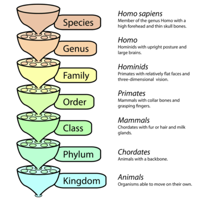
Linnaean System#
Linnaean System (1735): Carl Linnaeus formalized taxonomy by introducing a hierarchical system with specific ranks.
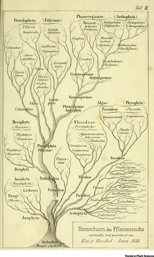
Darwin’s Theory of Evolution#
Darwin’s Theory of Evolution (1859): Charles Darwin’s “On the Origin of Species” proposed natural selection as a mechanism for evolution, fundamentally changing how organisms were understood in relation to one another. Darwin’s concept of common descent began to shape the idea of a “tree of life.”
With advances in comparative anatomy and embryology, with morphological and behavioral features, scientists began to construct early phylogenetic trees that depicted evolutionary relationships.
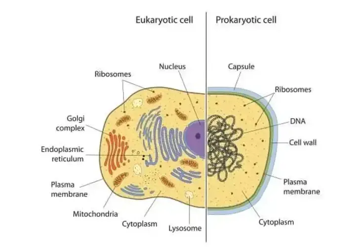
Eukaryote-Prokaryote Dichotomy#
Initial Classification (Late 19th Century): Early microbiologists, such as Louis Pasteur and Robert Koch, began differentiating between two major groups of life based on cellular organization: eukaryotes (organisms with complex cells containing a nucleus) and prokaryotes (simple, unicellular organisms without a nucleus).
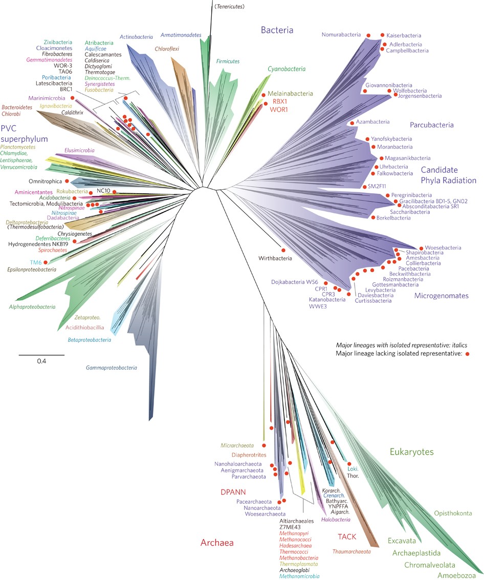
Three-Domain Theory#
In the 1970s, Carl Woese of the University of Illinois and his colleagues published the first “universal tree of life” by using the RNA tools. They presented the tree as three great trunks. Our own trunk, known as eukaryotes, includes animals, plants, fungi and protozoans. A second trunk included many familiar bacteria like Escherichia coli. The third trunk that Woese and his colleagues identified included little-known microbes that live in extreme places like hot springs and oxygen-free wetlands. Woese and his colleagues called this third trunk Archaea.
By 1990, Woese adopted the term “domain” for the three new branches of life. A major change to the Linnaean system was the addition of the “domain”. A domain is a taxon that is larger and more inclusive than the kingdom.
. . . .
In 2016, a team of scientists presented a new tree of life, illustrating the evolution of all living organisms. Their research revealed that bacteria constitute the majority of the branches in this tree. And they found that much of that diversity has been waiting in plain sight to be discovered, dwelling in river mud and meadow soils.
3.1.3.2 Human Microbiome#
Our human body contains about 10X as many microbes as human cells, including Bacteria, Archaea, viruses and Fungi.
Microbe community differs accross human body
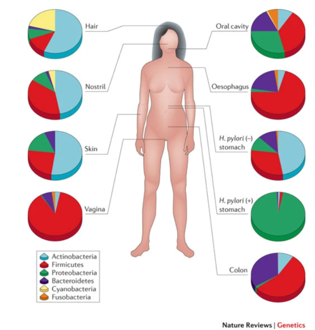
The human microbiome: at the interface of health and disease
First Introduction occurs at birth
Microbes provides enzymes for digestions and other compounds products such as Short-Chain Fatty Acids (SCFAs).
Carriage of microbial taxa varies while the metabolic pathways remain stable within the healthy population.
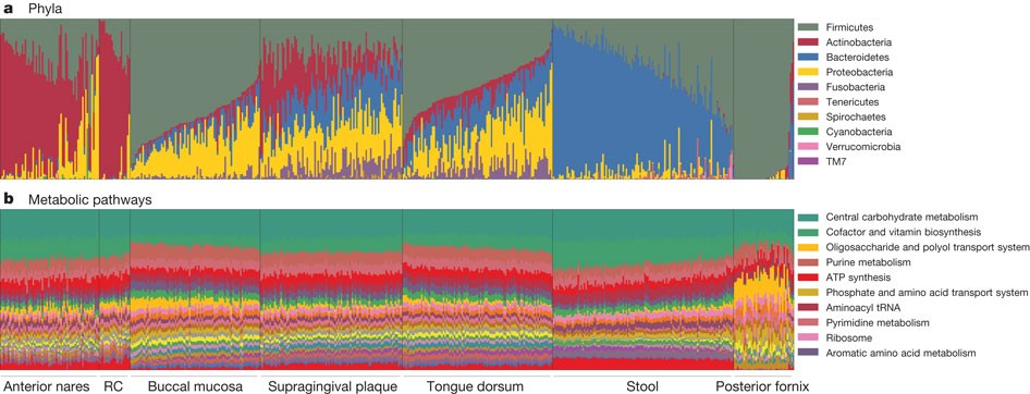
Structure, function and diversity of the healthy human microbiome
3.1.3.3 Principles of Amplicon Sequencing (16S/18S/ITS)#
If I have seen further, it is by standing on the shoulders of giants. – Sir Isaac Newton
Pioneer |
Main Contribution |
|---|---|
Carl Woese |
Propose the Archaea (a new domain of life) in 1977 through a pioneering phylogenetic taxonomy of 16S ribosomal RNA, a technique that has revolutionized microbiology. It is suggested that 16S rRNA gene can be used as a reliable molecular clock for Bacteria and Archaea because the 16S region contains conserved sequences for broad identification and variable regions that allow differentiation between species and strains. |
George E. Fox |
Collaboration with Carl Woese. Three-domain system Towards a natural system of organisms: proposal for the domains Archaea, Bacteria, and Eucarya. |
Pace, Norman R. |
The first characterization of the composition of a bacterial community (or microbiota) via the identification of 16S rRNA gene sequences without cell culture in 1985 |
So What is 16S rRNA?
Part of the subunit of prokaryotic ribosome
widely conserved (Bacteria and Archaea), but have hypervariable regions for differentiation.
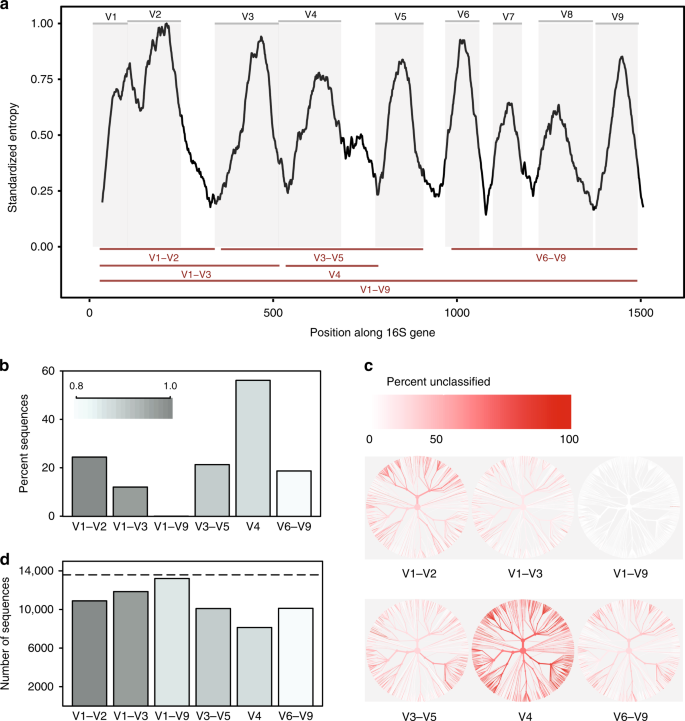
The choice of using different region is pivotal for optimizing phylogenetic resolution, cost-effectiveness, and microbial diversity assessment. You need to make a trade-off.
You may find the article below useful:
Other types of amplicon sequencing include 18S and ITS sequencing, which are used to study fungi.
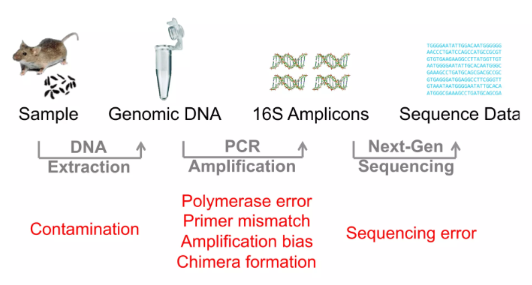
3.1.3.4 Common Amplicon Sequencing Steps#
The Schematic diagram describe the overview of 16s sequencing Heidi H. Kong, 2011:
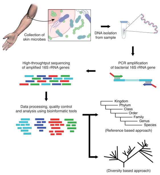
Common Amplicon Sequencing can be split into several steps:
Sample Preparation
This may involve adding enzymes to break down cell walls, applying heat to denature proteins, or using physical methods to separate cells from debris.
DNA Extraction
This is typically done using a DNA extraction kit, which uses a combination of chemical and physical methods to separate the DNA from other cellular components.
Library Preparation
Library preparation refers to the series of procedures that need to be taken to prepare the DNA for next generation sequencing, typically including 1) Amplification of the 16S rRNA gene. 2) Perform PCR to add molecular ‘barcodes’ to each cleaned DNA sample 3) clean DNA with magnetic microbeads
Sequencing
During sequencing, the DNA libraries are randomly amplified and sequenced using a combination of chemistry and optics. The resulting data generates short DNA sequences that can be aligned up to databases to identify which bacteria and archaea they belong to.
This Link from the most popular platform illumina introduce the NGS sequencing in a clear way.
3.1.4 Bioinformatics challenge: Sequencing and Alignment#
Terminology
Term |
Explain |
Note |
|---|---|---|
Reads Length |
The number of bases present in one read |
Longer reads can generally produce better results |
Sequencing Depth (or sometimes simply depth) |
The average number of times a given position in the genome is sequenced. |
More important in whole genome sequencing |
Number of reads |
Total amount of reads produced for a sample |
In 16s rRNA gene sequencing, we can consider number of reads the same as sampling depth, as we know which regrion are we targeting |
Coverage |
The proportion or percentage of a genome that has been sequenced at a certain depth. |
More important in whole genome sequencing |
3.1.4.1 Quality Control#
It is inevitable to HAVE some errors during 16S rRNA gene sequencing (Pay price for high number of information generated). But we can minimise these errors by using bioinformatics tools and proper experimental design.
So you must have got the basic understanding how the 16S or other amplicon sequencing can estimate and sample the microbial population in an efficient and accurate way. Now, let’s have a first glance at the sequencing output:
Find sample FASTQ file format,
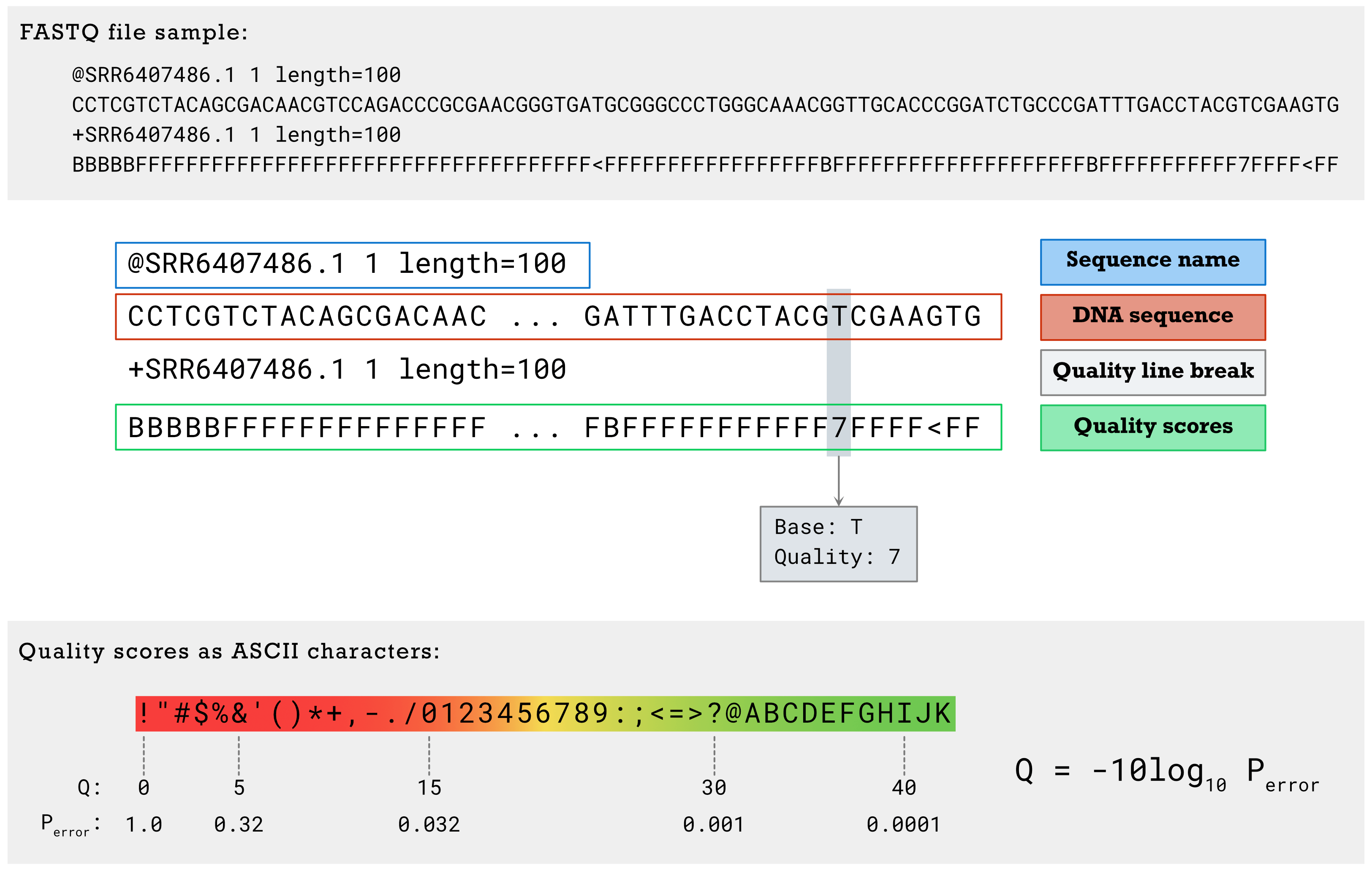
The quality score (Q) reflects in a logarithmic scale the probability that this particular base was called incorrectly (Perror). These scores can help identify low-confidence calls that are more likely to be erroneous. quality score equals to 20 (1 error happened in 100 bases) or 30 (more stringent, 1 error happened in 1000 bases) was normally set as the cutoff.
The question comes when we got the sequencing data,
Is the sequencing data with high quality?
Note
This is a complex question but worth to note when you are doing the analysis on the raw sequence data. Think about the following sub-questions:
Did you remove all the artifical sequence (e.g. the barcodes, the adpater for PCR)
Is your sequence of high sequencing quality?
Any contaminants present in my file?
Did you apply specific tools to correct the error induced during PCR? (e.g. DADA2 for 16S)
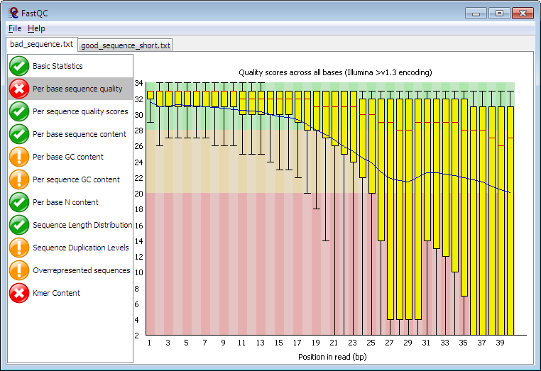
You may find more details about quality control here: Fastqc
3.1.4.2 Alignment#
After you believe you have got good quality of sequencing data, you may think about the following questions:
1.How to identify and classify the unknown bacteria sequence to known species (i.e. curated in database),
2.How to quantify the amount (abundance) of each unknown bacteria sequence.
Note
Like the traditional classification performed based on the traits and morphology, for sequencing and molecular classification, we typically seek to find similarity (aka, identity) between sequences. This procedure, called sequence alignment, is considered as the most essential step in bioinformatics.
Two commonly used sequence alignment algorithms are global alignment and local alignment.
Global alignment: Global alignment is a method of comparing two sequences, which aligns the entire length of the sequences by maximizing the overall similarity. This method is used when comparing sequences that are of the same length.
Local alignment: In local alignment, instead of attempting to align the entire length of the sequences, only the regions with the highest density of matches are aligned. This is useful for identifying short conserved regions in protein or nucleotide sequences.
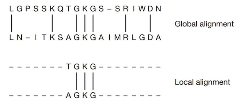
Global and Local Alignment of two sequences (Mount, D. W., 2001).
You will have practice about this mission in the practice session.
Example adopted from link
At present, you know how to identify the similarity between two sequences. Before we go deeper to the quantification part, we should first look at the possible issues we may meet.
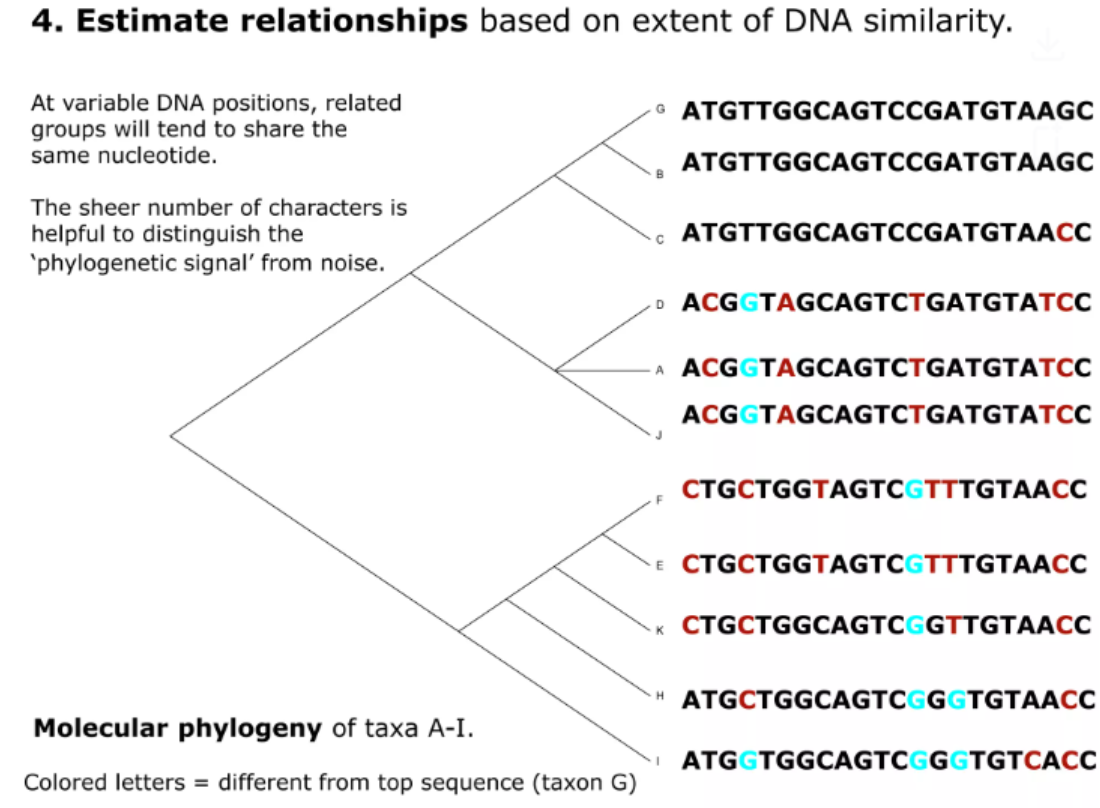
The goal for targeted sequencing is to determine its taxonomic origin based upon a potentially small number of variations relative to similar taxa. The results may be cofounded by single nucleotide variants (SNVs) caused by sequencer error, leading to a detection of a similar, but incorrect organism, or the false discovery of a new organism.
For millions of reads, it is computational intensive to analysis.
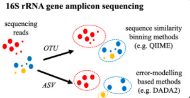
Scientists post a strategy to counter these two issues: find a proxy for microbial species. At the beginning, the proxy is based on the operational taxonomic units (OTUs), clusters of reads that differ by less than a fixed sequence dissimilarity threshold, most commonly 3% (i.e. 97% identity). The clustering method could be further divided into two strategies, 1) closed-reference methods - in which reads sufficiently similar to a sequence in a reference database are recruited into a corresponding OTU. 2) De novo methods - in which reads are grouped into OTUs as a function of their pairwise sequence similarities.
However, several disadvantages has been proposed:
Arbitrary Clustering: The 97% threshold is somewhat arbitrary and can lump distinct species together or split the same species.
Reproducibility Issues: Different software or parameters can produce different OTU clusters.
Low resolution: We can not fully believe the species-level resolution from this method.
In recent years, Amplicon Sequence Variants (ASVs) (100% idenitity sequence clustering and filter possible error by probability modelling) were proposed to minimize the effects. One of the most advantage is that ASVs can detect finer differences between sequences, providing more precise and accurate data, and do taxonomic assignment in a higher-resolution.
Tip
Difference between targeted sequencing and whole genome sequencing
In the context of whole genome sequencing, a small number of single nucleotide variants (SNVs) caused by sequencer error are unlikely to seriously confound an aligner and have little effect on the final attribution of the sequence. Targeted sequencing, where comparison of multiple similar sequences, rather than alignment across multiple genomes is the main operation, has the potential to be confounded by erroneous SNVs. This can result in misattribution of the sequence leading to either to detection of a similar, but incorrect organism, or the false discovery of a new organism.
After align the proxy (We call it Taxa in our tutorial) to the curated database, we may classify the taxa into different taxonomic ranks:
The taxonomic ranks used in this molecular classification system are:
Genus (About 93-97% identity)
Species (In general, > 99% identity depend on the targeted 16S region)
Each rank represents a level of classification
Tip
More advanced machine learning based taxonomic assignment method was also proposed e.g. naive bayes classifiers. You will learn more about machine learning in Professor Yin’s Lecture.
3.1.4.3 Pros and Cons of 16S rRNA Sequencing#
Pros:
Cost: Cost-effective.
Culture-independent: We only require DNA of the tested bacteria.
Cons:
While 16S rRNA sequencing is a powerful tool for identifying and characterizing microorganisms, it has some limitations in addition to strengths:
Taxonomic resolution: 16S rRNA sequencing targets a specific region of the bacterial genome that is relatively conserved across species but contains enough variation to differentiate between different taxa. However, this region may not always provide enough resolution to distinguish between closely related strains within a species due to limited genetic variability. Shotgun metagenomics sequencing works better which target the whole metagenome of the microbial community.
Identifying microbial functions: While 16S rRNA sequencing focuses solely on a single gene in bacteria and archaea, it is limited in its ability to reveal the full range of functional capacities exhibited by the microbes present in a sample. Shotgun metagenomics sequencing works better which target the whole metagenome of the microbial community.
Tip
The taxonomic resolution of 16S is dependent on region(s) targeted. If we can target the full length of the 16S rRNA gene (~1500bp), then we can probably increase the resolution to species-level identification. However, it can not be done with the next generation sequencing, in which we mainly provide short reads (~300bp).
Scientists are working on this issue, see Link here
3.1.5 Understand the Ecological Property of Microbiome: Alpha and Beta Diversity#
An ecological community consists of the collective populations of various species inhabiting a specific area. Each organism within this community occupies a unique ecological niche, encompassing
the physical environment they inhabit,
their utilization of available resources, and
their interactions with other organisms sharing the same space.
By defining their niche, organisms establish their role within the ecosystem, contributing to the intricate web of relationships that govern the functioning and dynamics of the community.
Different types of interspecific interactions have different effects on the two participants, which may be positive (+), negative (-), or neutral (0).
Interaction types |
Effect on species 1 |
Effect on species 2 |
|---|---|---|
Competition |
- |
- |
Predation |
+ |
- |
Mutualism |
+ |
+ |
Commensalism |
+ |
0 |
Parasitism |
+ |
- |
This is actually the area that underexplored and underdebate. Some scientists think the main interaction types between microbial species is competition rather than cooperation (Kevin R. Foster, 2012), while other disagree (Katharine Z. Coyte et al.).
One way to understand the diversity within a ecosystem or the dynamic stability of a certain microbial community is to use Alpha and Beta diversity.
Alpha diversity: The diversity within a particular niche or ecosystem (e.g. for example, human gut). Reduces the complexity of a multi-species community to a single integer that describes how many taxonomic units are present
Common Index, include:
the number of species (i.e., species richness) in that ecosystem.
The evenness (whether the microbial community was dominated by small proportion of the species.)
Beta diversity: A comparison of of diversity between ecosystems, usually measured as the amount of species change between the niche or ecosystems.
Common Index Could be split into two common types weighted and unweighted:
Unweightedmeans the Comparison between ecosystems only take the presence or absence of certain species into consideration: Jaccard Distance, Unweighted Unifrac distanceWeightedmeans the Comparison between ecosystems take the abundance information into consideration: Bray-Curtis Distance, Weighted Unifrac distance.
Jaccard Similarity = the size of the species intersection between divided by the size of the union species of the sample sets
Jaccard distance = 1 - Jaccard Similarity
Note
The idea that microorganisms exist solely as an independent unit evolved as it became clear that they form complex groups where species interact and communicate. High-throughput genome and metagenome analysis now offer powerful tools for studying both individual microbes and entire microbial communities in their natural environments.
Further Reading About Microbial Ecology:
3.1.5.1 Ordination#
Ordination is a statistical technique used in ecology to visualize and interpret complex multivariate data sets. It is particularly useful for exploring patterns and relationships among samples or variables in a dataset. Ordination methods aim to represent high-dimensional data in a lower-dimensional space while preserving the underlying structure and variation in the data.
here are various ordination techniques available, each with its own strengths and assumptions. Some common ordination methods include:
Principal Component Analysis (PCA): PCA is a widely used ordination method that reduces the dimensionality of the data by finding a set of orthogonal axes (principal components) that capture the maximum amount of variation in the data.
metric MultiDimensional Scaling (aka PCoA): the dissimilarities between samples are typically represented by a distance matrix, such as a Euclidean distance matrix or a Bray-Curtis dissimilarity matrix. The goal of PCoA is to find a set of axes (principal coordinates) that best capture the variation in the original dissimilarities.
Non-metric Multidimensional Scaling (NMDS): NMDS is a non-linear ordination method that aims to represent the dissimilarities between samples in a lower-dimensional space. It is often used when the data do not meet the assumptions of linear methods like PCA.
PCoA and NMDS is generally recommanded for microbiome data, therefore will be discussed below.
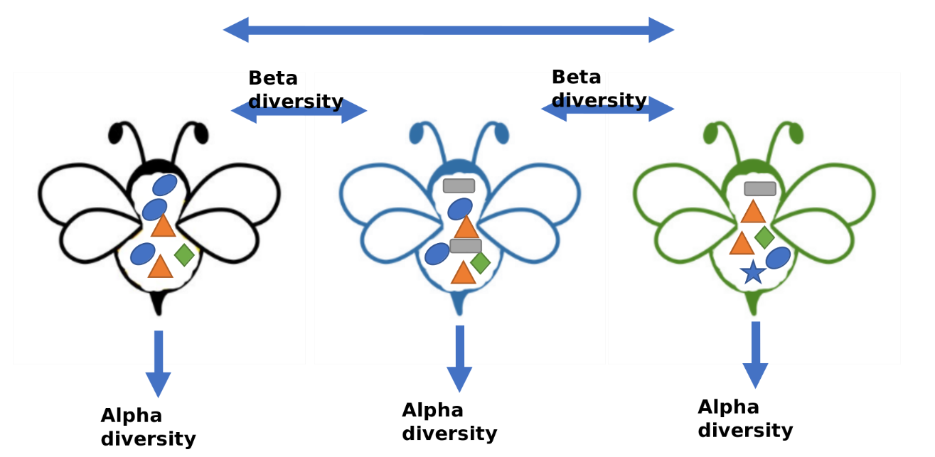
Case Exercise 6#
The figure describes the gut microbiota from our friends, honey maker - bumble bee, while different shapes represent for different bacteria. Could you calculate the alpha (species richness) for blue bee and green bee, beta diversity (Jaccard distance) between the blue bee and green bee?
Tip
Unifrac distance incorporates the phylogenetic distance between species into the comparison between ecosystems. Why take phylogenetic information into consideration can improve our understanding of the beta diversity?
3.2 Common Analysis in Microbiome study#
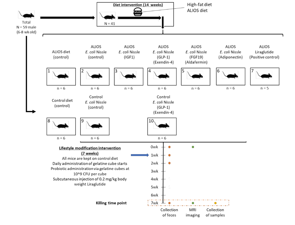
In this section, we will use the real microbiome data from Dr. Johnson et al. , NEEN project , which describe a control-treatment experiment design applied in mice to explore the function of first documented probiotics E.Coli Nissle in gut microbiota modulation. In this study, we applied 16s rRNA sequencing targting the v4 region.
3.2.1 Basic Experiment Design#
3.2.2 From Fasta File to Taxa Table#
We generated the data by the methodology published in the link.
This part will not be the main focus of this Course, but you may find the following link useful:
3.2.3 Import Data into R#
You will find the following data under documents/case7
Name |
Description |
Info |
|---|---|---|
taxa_table.tsv |
The ready-to-analysis microbial quantification matrix (row as Taxa, column as samples) generated by QIIME2 and dada2 pipeline |
784 taxa and 12 samples |
taxonomic_assignment_table.tsv |
The taxonomic assignment (row as Taxa, column as Taxonomic information) generated with greengene2 database |
784 taxa by 7 taxonomic ranks |
Phylogenetic Tree |
The ASVs phylogenetic tree |
Not provided |
sample_metadata_table.tsv |
The table indicating the sample-group relationship |
12 samples by Grouping variables |
Install the phyloseq package. It will take some time.
# Install phyloseq from Bioconductor
# if (!requireNamespace("BiocManager", quietly = TRUE))
#    install.packages("BiocManager")
# BiocManager::install("phyloseq")

# Install phyloseq from Github (Recommended)
# install.packages("devtools")
# devtools::install_github("phyloseq/joey711")

library(phyloseq)
sample_meta <- read.csv("../document/case7/sample_metadata_table.tsv",sep = "\t", row.names = 1)
sample_meta
| reference | Diet | Description | Group | |
|---|---|---|---|---|
| <int> | <chr> | <chr> | <chr> | |
| NEEN.011 | 11 | ALIOS diet | Group1 | CTRL |
| NEEN.012 | 12 | ALIOS diet | Group1 | CTRL |
| NEEN.013 | 13 | ALIOS diet | Group1 | CTRL |
| NEEN.014 | 14 | ALIOS diet | Group1 | CTRL |
| NEEN.015 | 15 | ALIOS diet | Group1 | CTRL |
| NEEN.016 | 16 | ALIOS diet | Group1 | CTRL |
| NEEN.021 | 21 | ALIOS diet | Group2 | EcN |
| NEEN.022 | 22 | ALIOS diet | Group2 | EcN |
| NEEN.023 | 23 | ALIOS diet | Group2 | EcN |
| NEEN.024 | 24 | ALIOS diet | Group2 | EcN |
| NEEN.025 | 25 | ALIOS diet | Group2 | EcN |
| NEEN.026 | 26 | ALIOS diet | Group2 | EcN |
table(sample_meta$Group) # Count the number of sample for each Group
CTRL  EcN
   6    6
taxa_table <- read.csv("../document/case7/taxa_table.tsv", sep = "\t", row.names = 1)
tail(taxa_table[1:6]) # You can find the Taxa id which is generated randomly to represent for different bacterial sequence (Taxa)
| NEEN.011 | NEEN.012 | NEEN.013 | NEEN.014 | NEEN.015 | NEEN.016 | |
|---|---|---|---|---|---|---|
| <int> | <int> | <int> | <int> | <int> | <int> | |
| bbaad0f397a1590db5c42bf1f40c8db9 | 0 | 13 | 0 | 12 | 0 | 22 |
| 1e040db0048bb4067f6d355cb45648dd | 99 | 116 | 149 | 59 | 121 | 302 |
| a6814253a38248cacced10ba5b2e3b1d | 143 | 60 | 109 | 80 | 394 | 1124 |
| d2be1254f5e7eb97bd42ec342d9cb11d | 6 | 0 | 0 | 6 | 0 | 0 |
| 45ec8d8b3f3f833abb943a394602ca67 | 0 | 0 | 0 | 0 | 0 | 0 |
| 2ce88e05f1919882b01289628bd3d156 | 0 | 0 | 9 | 6 | 21 | 20 |
You can use colSums() to calculate the Total Abundance (or called as sampling depth in our tutorial) of each sample
print(colSums(taxa_table))
NEEN.011 NEEN.012 NEEN.013 NEEN.014 NEEN.015 NEEN.016 NEEN.021 NEEN.022
   50047    49734    52780    47521    56489    56181    51627    51627
NEEN.023 NEEN.024 NEEN.025 NEEN.026
   52991    42890    48576    51663
Note
You can see that the total abundance varied accross samples. One of the important things for you to understand is that the abundance generated by the 16S rRNA sequencing (and probably other techniques based on sequencing) is highly dependent on the sampling depth (num of reads used in sequencing). Therefore, only sampling a fraction of the total population makes it invalid to compare between samples (We need some special statistical help). We will discuss it in next section 3.2.4.
taxonomic_assign_table <- read.csv("../document/case7/taxonomic_assignment_table.tsv", sep = "\t", row.names = 1)
tail(taxonomic_assign_table) # You may find NA present in the taxonomic assignment table
| Kingdom | Phylum | Class | Order | Family | Genus | Species | |
|---|---|---|---|---|---|---|---|
| <chr> | <chr> | <chr> | <chr> | <chr> | <chr> | <chr> | |
| bbaad0f397a1590db5c42bf1f40c8db9 | d__Bacteria | Firmicutes_A | Clostridia_258483 | Lachnospirales | Lachnospiraceae | NA | NA |
| 1e040db0048bb4067f6d355cb45648dd | d__Bacteria | Firmicutes_A | Clostridia_258483 | Lachnospirales | Lachnospiraceae | NA | NA |
| a6814253a38248cacced10ba5b2e3b1d | d__Bacteria | Firmicutes_A | Clostridia_258483 | Lachnospirales | Lachnospiraceae | NA | NA |
| d2be1254f5e7eb97bd42ec342d9cb11d | d__Bacteria | Firmicutes_A | Clostridia_258483 | Lachnospirales | Lachnospiraceae | NA | NA |
| 45ec8d8b3f3f833abb943a394602ca67 | d__Bacteria | Firmicutes_A | Clostridia_258483 | Lachnospirales | Lachnospiraceae | Kineothrix | Kineothrix sp000403275 |
| 2ce88e05f1919882b01289628bd3d156 | d__Bacteria | Firmicutes_A | Clostridia_258483 | Lachnospirales | Lachnospiraceae | NA | NA |
sort(unique(taxonomic_assign_table$Genus)) # Genus we have
- '14-2'
- '1XD42-69'
- '28-57-27'
- 'Acetatifactor'
- 'Acetitomaculum'
- 'Acutalibacter'
- 'Adlercreutzia_404199'
- 'Adlercreutzia_404218'
- 'Adlercreutzia_404257'
- 'Akkermansia'
- 'Alcanivorax_A'
- 'Aliidiomarina'
- 'Alistipes_A_871400'
- 'Alistipes_A_871404'
- 'Alkalibacterium'
- 'Alkalicoccus'
- 'Alkalimonas'
- 'Anaerotruncus'
- 'Angelakisella'
- 'Aquisalimonas'
- 'Avispirillum'
- 'Bacteroides_H'
- 'Bariatricus'
- 'Bifidobacterium_388775'
- 'Bilifractor'
- 'Bilophila'
- 'Borkfalkia'
- 'Butyribacter'
- 'Butyricicoccus_A_77030'
- 'BX12'
- 'C-19'
- 'C-53'
- 'CAG-269'
- 'CAG-273'
- 'CAG-314'
- 'CAG-41'
- 'CAG-485'
- 'CAG-56'
- 'CAG-632'
- 'CAG-873'
- 'CAG-95'
- 'Choladousia'
- 'Clostridium_AP'
- 'Clostridium_Q_134526'
- 'Clostridium_T'
- 'COE1'
- 'Conexibacter'
- 'Coprocola'
- 'Copromonas'
- 'Cryptobacteroides'
- 'D16-34'
- 'Demequina'
- 'Desulfovibrio_R_446353'
- 'Desulfurivibrio'
- 'Dethiobacter'
- 'Dubosiella'
- 'Duncaniella'
- 'Dysosmobacter'
- 'Ectothiorhodospira_607903'
- 'Emergencia'
- 'Enterenecus'
- 'Enterocloster'
- 'Enteroscipio'
- 'Erysipelatoclostridium'
- 'Escherichia_710834'
- 'Eubacterium_F'
- 'Eubacterium_G'
- 'Eubacterium_J'
- 'Eubacterium_R'
- 'Eubacterium_S'
- 'Evtepia'
- 'Faecalibaculum'
- 'Faecimonas'
- 'Faecousia'
- 'Fimenecus'
- 'GCA-002282575'
- 'GCA-2718595'
- 'Halofilum'
- 'Halolactibacillus'
- 'Halomonas_C_640989'
- 'Harryflintia'
- 'Holdemania'
- 'Hydrogenophaga_590395'
- 'Intestinimonas'
- 'Isachenkonia'
- 'Izemoplasma_B'
- 'JC017'
- 'Kineothrix'
- 'Kocuria'
- 'Lachnoclostridium_A_130679'
- 'Lachnoclostridium_B'
- 'Lachnospira'
- 'Lacrimispora'
- 'Lactobacillus'
- 'Lawsonibacter'
- 'Ligilactobacillus'
- 'Limivicinus'
- 'Limosilactobacillus'
- 'Luxibacter'
- 'Mailhella'
- 'Massilioclostridium'
- 'MD308'
- 'Merdibacter'
- 'Merdisoma'
- 'Methylophaga'
- 'Mucispirillum'
- 'Muribaculum'
- 'Nanosyncoccus'
- 'Natronospirillum'
- 'Nitrincola'
- 'NM07-P-09'
- 'Oceanicaulis'
- 'Odoribacter_865974'
- 'Oribacterium'
- 'Paludicola'
- 'Parabacteroides_B_862066'
- 'Paralachnospira'
- 'Paramuribaculum'
- 'Parasutterella'
- 'Pelethenecus'
- 'Peptococcus'
- 'Phocea'
- 'Planktosalinus'
- 'Planococcus'
- 'Porcincola'
- 'Prevotella'
- 'Pseudobutyricicoccus'
- 'Pseudomonas_D_641492'
- 'Pseudoxanthomonas_A_615337'
- 'QAMM01'
- 'QWKK01'
- 'Rhodobaculum'
- 'Rhodohalobacter'
- 'Robinsoniella'
- 'Roseinatronobacter'
- 'Ructibacterium'
- 'RUG12438'
- 'RUG762'
- 'Ruminiclostridium_E'
- 'Ruminococcus_B'
- 'Ruminococcus_C_58660'
- 'Ruthenibacterium'
- 'Salinarimonas'
- 'Salipaludibacillus_361384'
- 'Scatocola'
- 'Schaedlerella'
- 'Shewanella'
- 'Silanimonas_613110'
- 'SKVR01'
- 'Sodaliphilus'
- 'Sporofaciens'
- 'Staphylococcus'
- 'Streptococcus'
- 'Sulfurimonas'
- 'SZUA-442'
- 'TC1'
- 'Thioalkalivibrio_B'
- 'Thiomicrospira'
- 'Thiothrix_606507'
- 'Tindallia'
- 'Turicibacter'
- 'Turicimonas'
- 'UBA2658'
- 'UBA3263'
- 'UBA3282'
- 'UBA3789'
- 'UBA5905'
- 'UBA644'
- 'UBA6985'
- 'UBA7173'
- 'UBA737'
- 'UBA9414'
- 'UBA946'
- 'UBA9715'
- 'UMGS1071'
- 'UMGS1994'
- 'Ventrimonas'
- 'Ventrisoma'
- 'VRTS01'
- 'Wenzhouxiangella'
- 'Yoonia_491068'
- 'ZJ304'
Note
You will find some genus name, for example, “CAG-485” looks like the name generated by computer. Those are condidate genera name which we can identify the presence of certain organism by sequencing, however, we can not culture it so far, therefore, can not to do subsequent formal nomenculture.
Also, you may find the some genus name, for example, “Escherichia_710834”, looks loke a normal name plus a string of random number. Those are another example of why sequencing has revolutionized the microbiology study. GreenGene2 Database adopt the phylogenetic information from another important database GTDB. The former part from the example is, “Escherichia”. This is the name given by current formal nomenculture. However, based on the phylogenetic tree generated by the GTDB, the genera “Escherichia” might have the possibility (at least from the DNA sequence insights) to be split into subdivision or relocate to other genera.
tail(is.na(taxonomic_assign_table)) # whether the value in the matrix is NA with is.na()
| Kingdom | Phylum | Class | Order | Family | Genus | Species | |
|---|---|---|---|---|---|---|---|
| bbaad0f397a1590db5c42bf1f40c8db9 | FALSE | FALSE | FALSE | FALSE | FALSE | TRUE | TRUE |
| 1e040db0048bb4067f6d355cb45648dd | FALSE | FALSE | FALSE | FALSE | FALSE | TRUE | TRUE |
| a6814253a38248cacced10ba5b2e3b1d | FALSE | FALSE | FALSE | FALSE | FALSE | TRUE | TRUE |
| d2be1254f5e7eb97bd42ec342d9cb11d | FALSE | FALSE | FALSE | FALSE | FALSE | TRUE | TRUE |
| 45ec8d8b3f3f833abb943a394602ca67 | FALSE | FALSE | FALSE | FALSE | FALSE | FALSE | FALSE |
| 2ce88e05f1919882b01289628bd3d156 | FALSE | FALSE | FALSE | FALSE | FALSE | TRUE | TRUE |
Remember that the FALSE could be considered as 0, and the TRUE could be considered as 1.
print(colSums(is.na(taxonomic_assign_table))) # See how many NA present in each Taxonomic Ranks
Kingdom  Phylum   Class   Order  Family   Genus Species
      0       2       2       5      10     197     376
Warning
NA is a common symbol used in R to indicate the Missing Value. In our case, the missing value is because we did not have species or even genus level assignment for some of the taxa.
na.omit(df) - clean row with na
You need to take care of the missing value with caution.
We will replace NA values with the previous rank concatenated with “current rank” + “_no_rank”.
Note
Think about how to finish this mission if you are interested.
taxonomic_assign_table <- read.csv("../document/case7/taxonomic_assignment_table_revised.tsv", sep = "\t", row.names = 1) # we  will directly use the revised one
tail(taxonomic_assign_table)
| Kingdom | Phylum | Class | Order | Family | Genus | Species | |
|---|---|---|---|---|---|---|---|
| <chr> | <chr> | <chr> | <chr> | <chr> | <chr> | <chr> | |
| bbaad0f397a1590db5c42bf1f40c8db9 | d__Bacteria | Firmicutes_A | Clostridia_258483 | Lachnospirales | Lachnospiraceae | Lachnospiraceae_genus_no_rank | Lachnospiraceae_genus_no_rank_species_no_rank_OTU_bbaad0f397a1590db5c42bf1f40c8db9 |
| 1e040db0048bb4067f6d355cb45648dd | d__Bacteria | Firmicutes_A | Clostridia_258483 | Lachnospirales | Lachnospiraceae | Lachnospiraceae_genus_no_rank | Lachnospiraceae_genus_no_rank_species_no_rank_OTU_1e040db0048bb4067f6d355cb45648dd |
| a6814253a38248cacced10ba5b2e3b1d | d__Bacteria | Firmicutes_A | Clostridia_258483 | Lachnospirales | Lachnospiraceae | Lachnospiraceae_genus_no_rank | Lachnospiraceae_genus_no_rank_species_no_rank_OTU_a6814253a38248cacced10ba5b2e3b1d |
| d2be1254f5e7eb97bd42ec342d9cb11d | d__Bacteria | Firmicutes_A | Clostridia_258483 | Lachnospirales | Lachnospiraceae | Lachnospiraceae_genus_no_rank | Lachnospiraceae_genus_no_rank_species_no_rank_OTU_d2be1254f5e7eb97bd42ec342d9cb11d |
| 45ec8d8b3f3f833abb943a394602ca67 | d__Bacteria | Firmicutes_A | Clostridia_258483 | Lachnospirales | Lachnospiraceae | Kineothrix | Kineothrix sp000403275 |
| 2ce88e05f1919882b01289628bd3d156 | d__Bacteria | Firmicutes_A | Clostridia_258483 | Lachnospirales | Lachnospiraceae | Lachnospiraceae_genus_no_rank | Lachnospiraceae_genus_no_rank_species_no_rank_OTU_2ce88e05f1919882b01289628bd3d156 |
3.2.4 Normalization Issue#
We must first normalize our samples because sampling depth variations among samples can affect distance/dissimilarity measures. In this tutorial, we will focus on a common ways applied in 16S analysis: Rarefying (Or you can call it as subsampling to a given sampling depth).
Rarefying is the process of subsampling reads without replacement to a certain sampling depth. To have a basic understanding of the subsampling used in R. Let’s simplify the case into draw some letters from two boxes:
box1 <- c("A","A","A","B","B","B","B","C","C","D") # Set box1
box2 <- c("A","A","B","B","B","C","C") # Set box2
We will draw 5 letters from each of the boxes Without replacement. Without replacement means: once an letter is drawn it cannot be drawn again.
set.seed(2024) # set random seed to make sure the result is reproducible
sort(sample(box1, size = 5, replace = FALSE))
- 'A'
- 'A'
- 'B'
- 'B'
- 'C'
sort(sample(box2, size = 5, replace = FALSE))
- 'A'
- 'A'
- 'B'
- 'B'
- 'C'
The box1 and box2 have identical result when we randomly draw 5 letters. The result will change if you choose a different seed. However, if you draw many times, the probability of whether a spcific letter will be drawn will be stable. Let’s try:
draw_result = data.frame() # We will use dataframe to store the draw result
for (i in 1:1000){
   set.seed(i)
   tmp = sort(sample(box1, size = 5, replace = FALSE))
   draw_result = rbind(draw_result, tmp)
}
head(draw_result)
| X.A. | X.A..1 | X.B. | X.B..1 | X.C. | |
|---|---|---|---|---|---|
| <chr> | <chr> | <chr> | <chr> | <chr> | |
| 1 | A | A | B | B | C |
| 2 | A | B | B | C | D |
| 3 | A | A | B | B | B |
| 4 | A | B | B | C | C |
| 5 | A | A | A | B | C |
| 6 | A | B | B | C | C |
dim(draw_result)[1]*dim(draw_result)[2]
sum(draw_result == "A")/(dim(draw_result)[1]*dim(draw_result)[2])
sum(box1=="A")/length(box1)
Quite close to actual probability, right? This is an example of the power of computer simulation.
Warning
Some have argued that rarefying or rarefaction is “inadmissible” because it omits valid data (for example, you may see the missing of letter “D” in the box1 when you draw). Therefore, be aware of this situation when you are interesting in taxa with small amount. Other situations that may induced by rarefying.
The introduction of artificial uncertainty in the sub-sampling step,
The arbitrary selection of the minimum library size,
Challenges in estimating over-dispersion parameter.
Alternatives to rarefying: normalizing transformations (decostand in vegan) possible with variance stabilization (decostand and dispweight in vegan) and methods that are not sensitive to sample sizes
Keep the controversy in mind. Let’s go ahead.
Now, let’s show how can we do rarefy on our microbiome data:
library(vegan) # load vegan package
Loading required package: permute
Loading required package: lattice
This is vegan 2.6-8
Vegan accept the transposed taxa table (row as sample, column as taxa), so lets transpose our taxa table first
transposed_taxa_table <- t(taxa_table)

raremax <- 25000 # get the minimum sampling

vegan::rarecurve(transposed_taxa_table, step = 10, sample = raremax, col = "lightgreen", cex = 0.6)

# Step size for sample sizes in rarefaction curves.
Warning message in vegan::rarecurve(transposed_taxa_table, step = 10, sample = raremax, :
“most observed count data have counts 1, but smallest count is 2”
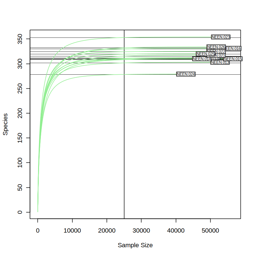
As you can see in the Figure above, the alpha diversity (species richness in this case) did not change significantly when the sequencing depth larger than 25000 (i.e. reaches a plateau). We consider the sequencing depth is sufficient to cover what we need. As we want to retain as many as the data we produced when trying to reduce the sampling bias, we will choose minimum sampling depth as the even sampling depth used accross the sample. We will imply the rarefy_even_depth function used in phyloseq package for this purpose.
3.2.5 Phyloseq Object#
Phyloseq is a widely used R object to store the 16s data as well as other metagenomics data.
You will find 3 main objects embedded in the phyloseq object in this tutorial:
otu_table: similar to taxa_table
tax_table: similar to taxonomic_assign_table
sample_data: similar to sample_meta
head(otu_table(taxa_table, taxa_are_rows = T)) # convert the taxa_table into otu_table object
| NEEN.011 | NEEN.012 | NEEN.013 | NEEN.014 | NEEN.015 | NEEN.016 | NEEN.021 | NEEN.022 | NEEN.023 | NEEN.024 | NEEN.025 | NEEN.026 | |
|---|---|---|---|---|---|---|---|---|---|---|---|---|
| 3af64985583451cceeb3901d043bfd73 | 0 | 19 | 0 | 0 | 0 | 0 | 0 | 0 | 0 | 0 | 0 | 0 |
| a57944ffff8ec2097b06e45a616f907d | 0 | 0 | 0 | 0 | 0 | 0 | 0 | 0 | 0 | 0 | 0 | 0 |
| a69c0a328e1b282389062478c5d49c3a | 68 | 82 | 96 | 45 | 27 | 24 | 27 | 45 | 34 | 17 | 9 | 6 |
| 7d02f99e2ea00512b055a4e70f84c18b | 111 | 64 | 29 | 40 | 768 | 513 | 260 | 66 | 25 | 21 | 14 | 15 |
| 54a43d2113c13203e813d22b17f3f370 | 47 | 55 | 50 | 25 | 33 | 56 | 84 | 29 | 16 | 18 | 16 | 22 |
| e127450ed2ad1088a651c6a3f8a405b3 | 0 | 5 | 0 | 3 | 0 | 0 | 0 | 0 | 0 | 0 | 6 | 0 |
head(tax_table(as.matrix(taxonomic_assign_table))) # convert the taxonomic_assign_table into tax_table object
| Kingdom | Phylum | Class | Order | Family | Genus | Species | |
|---|---|---|---|---|---|---|---|
| 3af64985583451cceeb3901d043bfd73 | d__Bacteria | Bacteroidota | Bacteroidia | Bacteroidales | Muribaculaceae | UBA7173 | UBA7173 sp002491305 |
| a57944ffff8ec2097b06e45a616f907d | d__Bacteria | Bacteroidota | Bacteroidia | Bacteroidales | Muribaculaceae | Sodaliphilus | Sodaliphilus pleomorphus |
| a69c0a328e1b282389062478c5d49c3a | d__Bacteria | Bacteroidota | Bacteroidia | Bacteroidales | Muribaculaceae | CAG-485 | CAG-485 sp900547755 |
| 7d02f99e2ea00512b055a4e70f84c18b | d__Bacteria | Bacteroidota | Bacteroidia | Bacteroidales | Marinifilaceae | Odoribacter_865974 | Odoribacter laneus |
| 54a43d2113c13203e813d22b17f3f370 | d__Bacteria | Bacteroidota | Bacteroidia | Bacteroidales | Marinifilaceae | Odoribacter_865974 | Odoribacter splanchnicus |
| e127450ed2ad1088a651c6a3f8a405b3 | d__Bacteria | Bacteroidota | Bacteroidia | Bacteroidales | Marinifilaceae | Odoribacter_865974 | Odoribacter splanchnicus |
head(sample_data(sample_meta))
| reference | Diet | Description | Group | |
|---|---|---|---|---|
| <int> | <chr> | <chr> | <chr> | |
| NEEN.011 | 11 | ALIOS diet | Group1 | CTRL |
| NEEN.012 | 12 | ALIOS diet | Group1 | CTRL |
| NEEN.013 | 13 | ALIOS diet | Group1 | CTRL |
| NEEN.014 | 14 | ALIOS diet | Group1 | CTRL |
| NEEN.015 | 15 | ALIOS diet | Group1 | CTRL |
| NEEN.016 | 16 | ALIOS diet | Group1 | CTRL |
Then Merge them into a phyloseq object
physeq <- phyloseq(otu_table(taxa_table, taxa_are_rows = T),
                   tax_table(as.matrix(taxonomic_assign_table)),
                   sample_data(sample_meta) )
physeq # You can see a very nice summary of the current data
phyloseq-class experiment-level object
otu_table()   OTU Table:         [ 784 taxa and 12 samples ]
sample_data() Sample Data:       [ 12 samples by 4 sample variables ]
tax_table()   Taxonomy Table:    [ 784 taxa by 7 taxonomic ranks ]
phyloseq package provide many useful wrapper function to analysis the phyloseq object, like:
print(sample_sums(physeq)) # Quite familiar, right? this function output the total taxa abundance for each sample
NEEN.011 NEEN.012 NEEN.013 NEEN.014 NEEN.015 NEEN.016 NEEN.021 NEEN.022
   50047    49734    52780    47521    56489    56181    51627    51627
NEEN.023 NEEN.024 NEEN.025 NEEN.026
   52991    42890    48576    51663
sample_names(physeq)
- 'NEEN.011'
- 'NEEN.012'
- 'NEEN.013'
- 'NEEN.014'
- 'NEEN.015'
- 'NEEN.016'
- 'NEEN.021'
- 'NEEN.022'
- 'NEEN.023'
- 'NEEN.024'
- 'NEEN.025'
- 'NEEN.026'
rank_names(physeq)
- 'Kingdom'
- 'Phylum'
- 'Class'
- 'Order'
- 'Family'
- 'Genus'
- 'Species'
sample_variables(physeq)
- 'reference'
- 'Diet'
- 'Description'
- 'Group'
Keep only taxa with KNOWN Phylum
physeq <- subset_taxa(physeq, Phylum != "d__Bacteria_phylum_no_rank") # Phylum is one of the column from tax_table().
physeq
phyloseq-class experiment-level object
otu_table()   OTU Table:         [ 782 taxa and 12 samples ]
sample_data() Sample Data:       [ 12 samples by 4 sample variables ]
tax_table()   Taxonomy Table:    [ 782 taxa by 7 taxonomic ranks ]
physeq.rarefy = rarefy_even_depth(physeq,
                                  replace = F,
                                  sample.size = min(sample_sums(physeq)) , # sample_sums() function from ph
                                  rngseed = 20230927) # random seed, so that the result is reproducible
print(sample_sums(physeq.rarefy))
`set.seed(20230927)` was used to initialize repeatable random subsampling.
Please record this for your records so others can reproduce.
Try `set.seed(20230927); .Random.seed` for the full vector
...
186OTUs were removed because they are no longer
present in any sample after random subsampling
...
NEEN.011 NEEN.012 NEEN.013 NEEN.014 NEEN.015 NEEN.016 NEEN.021 NEEN.022
   42877    42877    42877    42877    42877    42877    42877    42877
NEEN.023 NEEN.024 NEEN.025 NEEN.026
   42877    42877    42877    42877
3.2.5 Calculate the Taxa-based Diversity#
Each of the Taxa represent a microbial sequence, although some of them hasn’t been fully assigned with the taxonomic ranks. This is possibly because the unassigned taxa are new species that the database hasn’t fully curated.
Phyloseq help us to the alpha diversity analysis in a easy way.
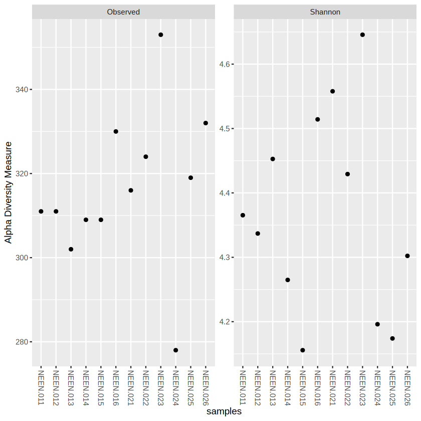
plot_richness(physeq.rarefy, measures=c("Observed", "Shannon")) # measures could be used to determine which alpha diversity you want to include
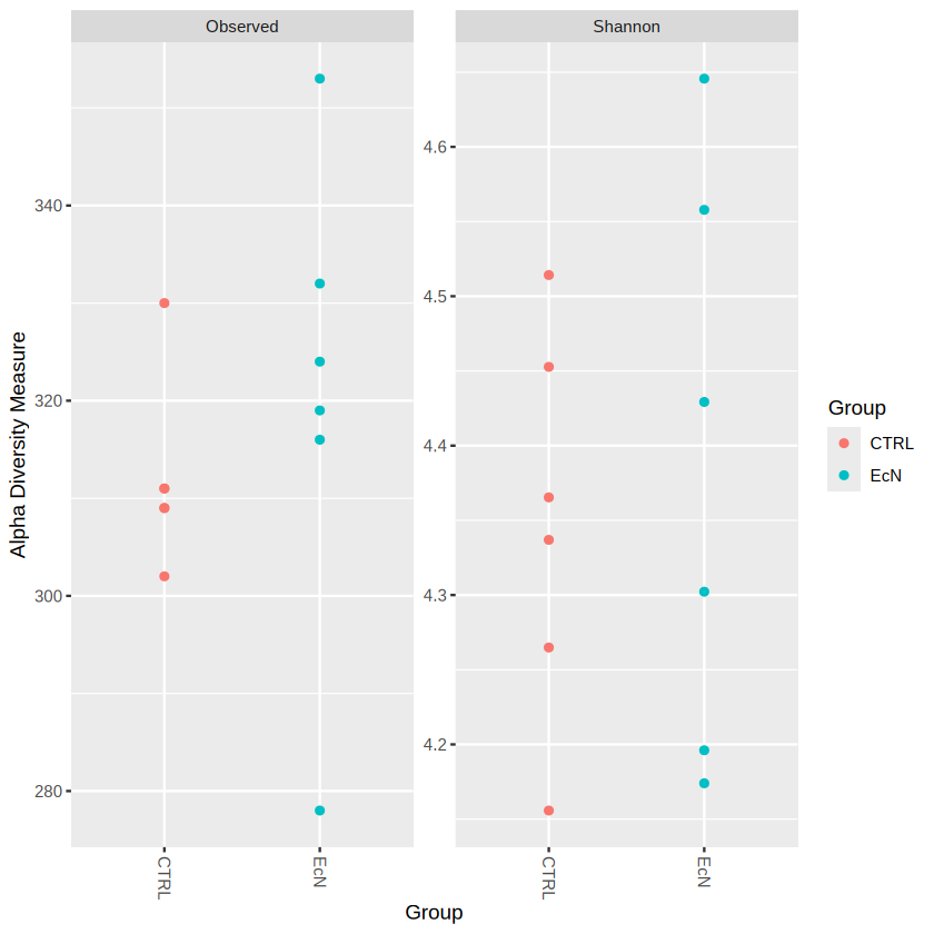
plot_richness(physeq.rarefy, x="Group", color="Group", measures=c("Observed", "Shannon")) # we set x as "Group", "Group" is the information in sample_data() object
We could add some extra ggplot2 code to modify the output
library(ggplot2)
plot_richness(physeq.rarefy, x="Group", color="Group", measures=c("Observed", "Shannon")) +
    geom_boxplot(aes(color=Group)) # geom_* --- is a common syntax used in ggplot2
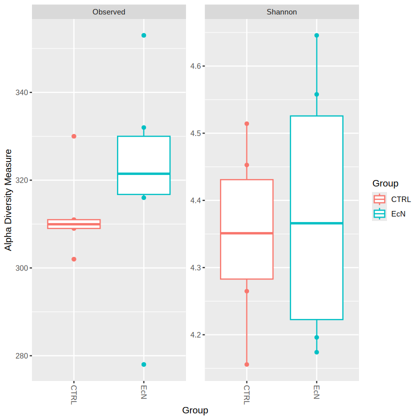
We could probably see that EcN have generally higher observed species (species richness) than CTRL group. You can also observe the Taxonomic Composition by barplot.
plot_bar(physeq.rarefy, fill="Phylum")
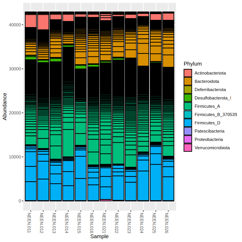
The bar plot looks quite ugly, right? Make the bar plot nicer by removing the taxa boundaries. The plot function in phyloseq actually code based on ggplot2, similarly, we can add some ggplot2 code to modify it.
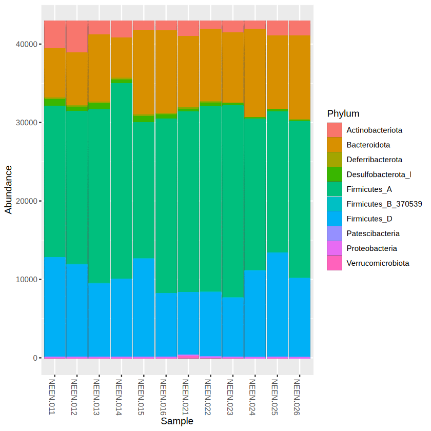
library(ggplot2)
plot_bar(physeq.rarefy, fill = "Phylum") +
  geom_bar(aes(color=Phylum, fill=Phylum), stat="identity", position="stack")
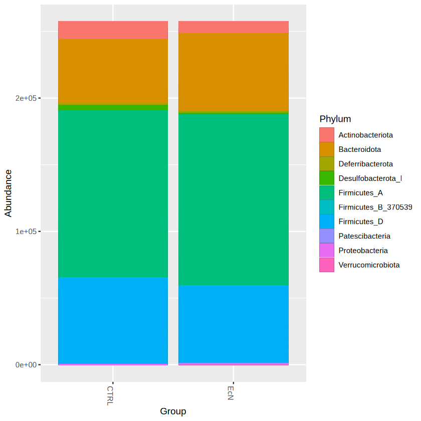
library(ggplot2)
plot_bar(physeq.rarefy, x = "Group", fill = "Phylum") +
  geom_bar(aes(color=Phylum, fill=Phylum), stat="identity", position="stack")
  # stat = "identity": performs no extra computation on the data
  # position = "stack": automatically stack values in reverse order of the group aesthetic, which for bar charts is usually defined by the fill aesthetic
We will then do multivariate analysis based on Bray-Curtis distance and Non-metric Multidimensional Scaling (NMDS) ordination.
physeq.ord <- ordinate(physeq.rarefy, "NMDS", "bray")
Square root transformation
Wisconsin double standardization
Run 0 stress 0.08689726
Run 1 stress 0.08689727
... Procrustes: rmse 4.48701e-05  max resid 0.000109021
... Similar to previous best
Run 2 stress 0.08689726
... Procrustes: rmse 1.847964e-05  max resid 4.123059e-05
... Similar to previous best
Run 3 stress 0.08689726
... New best solution
... Procrustes: rmse 6.799869e-06  max resid 1.058429e-05
... Similar to previous best
Run 4 stress 0.08689727
... Procrustes: rmse 2.327513e-05  max resid 5.535294e-05
... Similar to previous best
Run 5 stress 0.1213845
Run 6 stress 0.1213846
Run 7 stress 0.3244416
Run 8 stress 0.08689726
... Procrustes: rmse 5.540047e-06  max resid 8.579548e-06
... Similar to previous best
Run 9 stress 0.08689727
... Procrustes: rmse 1.625888e-05  max resid 3.099486e-05
... Similar to previous best
Run 10 stress 0.08689726
... Procrustes: rmse 7.135722e-07  max resid 1.273998e-06
... Similar to previous best
Run 11 stress 0.1213845
Run 12 stress 0.1213845
Run 13 stress 0.08689726
... Procrustes: rmse 3.255696e-06  max resid 7.64139e-06
... Similar to previous best
Run 14 stress 0.08689726
... Procrustes: rmse 1.430007e-06  max resid 2.54728e-06
... Similar to previous best
Run 15 stress 0.08689726
... Procrustes: rmse 1.181552e-05  max resid 2.89592e-05
... Similar to previous best
Run 16 stress 0.08689726
... New best solution
... Procrustes: rmse 2.873369e-06  max resid 6.851487e-06
... Similar to previous best
Run 17 stress 0.08689726
... New best solution
... Procrustes: rmse 3.405353e-06  max resid 8.257777e-06
... Similar to previous best
Run 18 stress 0.1213845
Run 19 stress 0.347306
Run 20 stress 0.08689726
... Procrustes: rmse 9.14899e-06  max resid 2.112381e-05
... Similar to previous best
*** Best solution repeated 2 times
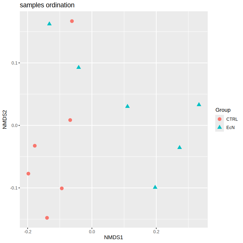
plot_ordination(physeq.rarefy, physeq.ord, type="samples", color="Group", shape= "Group",
                  title="samples ordination") + geom_point(size=3)
Note
You can also extract the data that we used to plot this picture by
first assign the result to a object
plot <- plot_ordination(...)Then the data could be found using
plot$data
Based on the ordination results, we can observe a clear separation between the samples in CTRL and EcN, especially in NMDS1. Remember in Section 3.1, we have discussed that the ordination techniques could condense the main variation between samples in a reduced dimension (2 in our case, i.e. NMDS1, NMDS2). The difference in NMDS1 indicating a noticable difference in the microbial composition. To gain statistical support, we will also apply PERMOANOVA to the dataset to test the significance based on the bray-curtis distance matrix.
PERmutational Multivariate ANalysis of VAriance (PERMANOVA) is a permutation-based technique – it makes no distributional assumptions about multivariate normality or homogeneity of variances. In essence, similar to ANOVA, the PERMANOVA is designed for compares the variation between groups to the variation within groups.
To do so, we need to extract the otu_table and sample data from the phyloseq object.
adonis_taxa <- t(otu_table(physeq.rarefy))
adonis_sample_data <- data.frame(sample_data(physeq.rarefy))
vegan::adonis2( formula = adonis_taxa ~ Group, data = adonis_sample_data, method = "bray")
# In this case, the left hand side of formula is the abundance matrix, while the right hand side is the variable that you want to associated with
| Df | SumOfSqs | R2 | F | Pr(>F) | |
|---|---|---|---|---|---|
| <dbl> | <dbl> | <dbl> | <dbl> | <dbl> | |
| Model | 1 | 0.2830608 | 0.2795537 | 3.880284 | 0.002 |
| Residual | 10 | 0.7294848 | 0.7204463 | NA | NA |
| Total | 11 | 1.0125457 | 1.0000000 | NA | NA |
Based on the result from PERMANOVA, we can confidently draw the conclusion that EcN has significantly alter the bacteria community.
3.2.6 Differential Abundant Analysis#
Indeed, our E.Coli Nissle can significantly change the microbial community. But how to gain more specific insights about which bacteria increased or decreased by our treatment? There are different tools including LEfSe, ANCOMBC, ANCOMBC2, MaAsLin2 and DESeq2 etc. Every tools rely on different assumptions about the data. In this tutorial, to keep consistent with the NEEN project, we will apply ANCOMBC to the differential abundant analysis.
# ========= Install ==========

# if (!require("BiocManager", quietly = TRUE))
#    install.packages("BiocManager")

# BiocManager::install("ANCOMBC", version = "2.6.0")

library("ANCOMBC")
packageVersion("ANCOMBC")
[1] ‘2.6.0’
Note
The R version used in this tutorial is 4.4.
physeq
phyloseq-class experiment-level object
otu_table()   OTU Table:         [ 782 taxa and 12 samples ]
sample_data() Sample Data:       [ 12 samples by 4 sample variables ]
tax_table()   Taxonomy Table:    [ 782 taxa by 7 taxonomic ranks ]
# ANCOMBC designed the algorithm to fix the sampling depth bias, therefore, we could directly use the un-rarefied physeq

ancombc_result = ancombc(phyloseq = physeq,
                tax_level = "Genus",
                formula = "Group",   # formula can be used to add more cofounder, see ?ANCOMBC
                p_adj_method = "BH", # p value adjustment method
                prv_cut = 0.10,      # Prevalence cutoff
                lib_cut = 1000,
                group = "Group",     # The Group variable
                struc_zero = TRUE, neg_lb = TRUE, tol = 1e-5,
                max_iter = 100, conserve = TRUE, alpha = 0.05, global = TRUE,
                n_cl = 1, verbose = TRUE)
'ancombc' has been fully evolved to 'ancombc2'.
Explore the enhanced capabilities of our refined method!
Warning message:
“The group variable has < 3 categories
The multi-group comparisons (global/pairwise/dunnet/trend) will be deactivated”
Obtaining initial estimates ...
Estimating sample-specific biases ...
Loading required package: foreach
Loading required package: rngtools
ANCOM-BC primary results ...
Merge the information of structural zeros ...
Note that taxa with structural zeros will have 0 p/q-values and SEs
names(table(sample_data(physeq)[,"Group"]))[1]
# We need to get the p value and lfc used for the group
level1 = names(table(sample_data(physeq)[,"Group"]))[1] # In this case, CTRL
level2 = names(table(sample_data(physeq)[,"Group"]))[2] # In this case, EcN

# typically, the column name would be varname + level2
column_name = paste0("Group", level2)

# Extract differentially abundant taxa
# The fold change defined in ANCOMBC is level2/level1

diff_abundant_taxa_lfc <- ancombc_result$res$lfc
diff_abundant_taxa_lfc$FC <-  exp(ancombc_result$res$lfc[, column_name]) # this is because the ANCOMBC employ a natural log transformation


diff_abundant_taxa_p <- ancombc_result$res$p_val
diff_abundant_taxa_p$P <-  ancombc_result$res$p_val[, column_name]
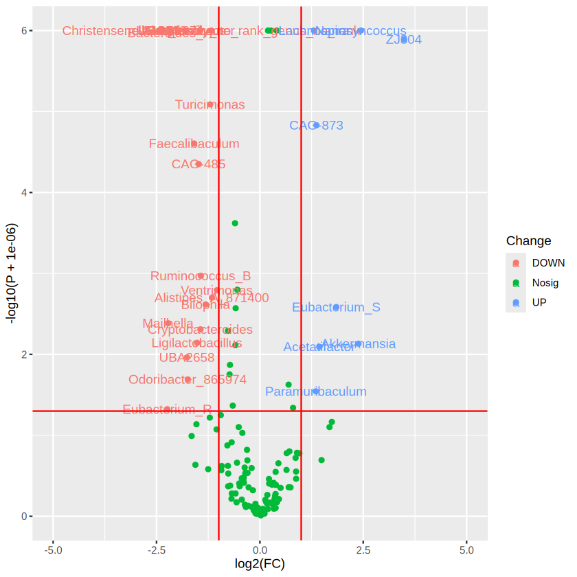
then, we will introduce a plot commonly used in the field, volcano plot.
# taxa_species_relation <- tax_tab
taxa_p <- diff_abundant_taxa_p[,c("taxon","P")]
taxa_fc <- diff_abundant_taxa_lfc[,c("taxon","FC")]

merged_res = merge(taxa_p,taxa_fc )

# add a column of NAs
merged_res$Change <- "Nosig"
# if log2Foldchange > 1 and pvalue < 0.05, set as "UP"
merged_res$Change[log2(merged_res$FC) > 1 & merged_res$P < 0.05] <- "UP"
# if log2Foldchange < -0.6 and pvalue < 0.05, set as "DOWN"
merged_res$Change[log2(merged_res$FC) < -1 & merged_res$P < 0.05] <- "DOWN"

# Add a column for further Text label
merged_res$label <- merged_res$taxon
merged_res$label[merged_res$Change == "Nosig"] <- "" # Therefore, we do not want the label for not significant species

# Make sure you install package "DT"
# Display
DT::datatable(merged_res, caption = "P value and Fold Changes from the Primary Result")
head(merged_res)
| taxon | P | FC | Change | label | |
|---|---|---|---|---|---|
| <chr> | <dbl[,1]> | <dbl> | <chr> | <chr> | |
| 1 | 14-2 | 0.3294346226 | 0.7636420 | Nosig | |
| 2 | 1XD42-69 | 0.2675192797 | 1.5627751 | Nosig | |
| 3 | Acetatifactor | 0.0080507628 | 2.7043133 | UP | Acetatifactor |
| 4 | Acetitomaculum | 0.3532689676 | 0.7583377 | Nosig | |
| 5 | Acutalibacter | 0.0002387997 | 0.6594520 | Nosig | |
| 6 | Acutalibacteraceae_genus_no_rank | 0.4376746016 | 1.6212742 | Nosig |
write.csv(merged_res, file = "../document/case7/final_res.csv")
library("ggplot2")
ggplot(data=merged_res, aes(x=log2(FC), y= -log10(P + 0.000001), color = Change)) +  # + 0.000001 was set to remove p value = 0
   geom_point() +
   geom_text(aes(label = label))  + # add taxa information
   geom_vline(xintercept=c(-1, 1), col="red") +
   geom_hline(yintercept=-log10(0.05), col="red") +
   scale_x_continuous(limits = c(-5,5)) + # set the parameter for x axis
   scale_y_continuous(limits = c(0,6))    # set the parameter for y axis
# You may find the graph quite ugly, try this instead

library("ggplot2")
library("ggrepel")
ggplot(data=merged_res, aes(x=log2(FC), y= -log10(P + 0.000001), color = Change)) +  # + 0.000001 was set to remove p value = 0
   geom_point() +
   # geom_text(aes(label = label))  +
   geom_text_repel(aes(label = label),max.overlaps = 200) + # add taxa information with flexible position
   geom_vline(xintercept=c(-1, 1), col="red") +
   geom_hline(yintercept=-log10(0.05), col="red") +
   scale_x_continuous(limits = c(-5,5)) + # set the parameter for x axis
   scale_y_continuous(limits = c(0,7))    # set the parameter for y axis
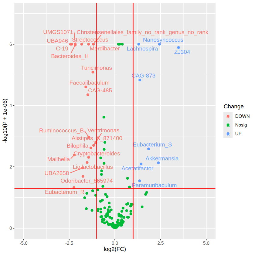
ggplot2 is a powerful tool to learn for visualization!
3.2.7 Correlation Analysis#
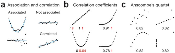
Normally, Correlation and Association are two terms can be used interchangeably. But they have some tiny but important difference that worth to note when interpret the results.
Association: A more vague term used to describe a relationship (linear or non-linear) between two variables.
Correlation: A certain type of (usually linear) association between two variables.
What is a linear relationship?
A linear relationship (or linear association) is a statistical term used to describe a straight-line relationship between two variables. In math, we can write it as y = mx + b. where: m=slope, b = intercept
Basically, we have two main types of data: One is categorical (like girl and boy; or disease and healthy), another one is continuous data (like the height or the proportion of fatty liver). The differential abundant analysis that we have discussed before is actually a kind of association analysis, which mainly focus on the association between continous (the abundance of certain bacteria) and categorical data.
In this section, we will focus on the correlation analysis which is normally used to describe the relationship between two continous data, such as the linear relationship between the height and the weight for each person.
For both association/correlation, we can describe it as either positive or negative association.
Negative: As one variable increases, the other will increase (move in the same direction)
Positive: As one variable increases, the other will decrease (move in the oppositive direction)
For correlation, we can use some statistics, i.e. correlation coefficient, to describe the STRENGTH of correlation. The range of correlation coefficient is [-1,1]. Where the -1 indicates the strongest negative correlation, 1 indicates the strongest positive correlation.
Different Statistics rely on different assumptions, Here is the assumptions for two commonly used:
Pearson’s r:
Data from both variables follow normal distributions
You expect a linear relationship between the two variables.
Paired observations
Spearman’s rho:
Not have any assumptions on the distribution, will use the rank
There is a monotonic relationship between the two variables.
Paired observations
Let’s try with the metadata provided by Dr. Johnson Lok for the NEEN data, in which, we measure the short-chain fatty acid level from either plasma and face and the body weight , etc after we sacrifice the mice.
meta_endpoints_data <- read.csv("../document/case9/Meta_endpoint_table.tsv",sep = "\t",
row.names = 1 # set the first column as the rownames index
)
head(meta_endpoints_data)
| NEEN.011 | NEEN.012 | NEEN.013 | NEEN.014 | NEEN.015 | NEEN.016 | NEEN.021 | NEEN.022 | NEEN.023 | NEEN.024 | ⋯ | NEEN.033 | NEEN.034 | NEEN.035 | NEEN.036 | NEEN.051 | NEEN.052 | NEEN.053 | NEEN.054 | NEEN.055 | NEEN.056 | |
|---|---|---|---|---|---|---|---|---|---|---|---|---|---|---|---|---|---|---|---|---|---|
| <dbl> | <dbl> | <dbl> | <dbl> | <dbl> | <dbl> | <dbl> | <dbl> | <dbl> | <dbl> | ⋯ | <dbl> | <dbl> | <dbl> | <dbl> | <dbl> | <dbl> | <dbl> | <dbl> | <dbl> | <dbl> | |
| Body weight (g) | 30.20000000 | 3.110000e+01 | 3.430000e+01 | 36.000000 | 43.90000000 | 43.00000000 | 34.900000 | 29.000000 | 32.90000000 | 37.70000000 | ⋯ | 3.610000e+01 | 32.000000 | 36.70000 | 32.500000 | 32.90000 | 31.300000 | 32.400000 | 3.080000e+01 | 3.460000e+01 | 3.480000e+01 |
| Body weight loss (%) | -0.66666667 | 3.715170e+00 | 3.107345e+00 | 7.216495 | -3.78250591 | -7.50000000 | 4.644809 | -2.836879 | -0.30487805 | -3.00546448 | ⋯ | 3.989362e+00 | 5.325444 | 4.92228 | 6.876791 | 5.45977 | 9.537572 | 5.263158 | 6.097561e+00 | 6.738544e+00 | 4.918033e+00 |
| Body weight loss (g) | -0.20000000 | 1.200000e+00 | 1.100000e+00 | 2.800000 | -1.60000000 | -3.00000000 | 1.700000 | -0.800000 | -0.10000000 | -1.10000000 | ⋯ | 1.500000e+00 | 1.800000 | 1.90000 | 2.400000 | 1.90000 | 3.300000 | 1.800000 | 2.000000e+00 | 2.500000e+00 | 1.800000e+00 |
| Liver weight (mg) | 1700.00000000 | 1.480000e+03 | 1.650000e+03 | 1780.000000 | 2443.00000000 | 2197.00000000 | 1740.000000 | 1360.000000 | 1660.00000000 | 2010.00000000 | ⋯ | 1.850000e+03 | 1690.000000 | 1850.00000 | 1620.000000 | 1660.00000 | 1380.000000 | 1490.000000 | 1.740000e+03 | 1.860000e+03 | 1.700000e+03 |
| MRI fat index | 0.03815241 | 6.350756e-02 | 3.607113e-02 | NA | 0.12080000 | 0.14480000 | NA | NA | 0.06871337 | 0.09788389 | ⋯ | 4.194388e-02 | NA | NA | NA | NA | NA | NA | 3.169522e-02 | 3.825281e-02 | 3.357185e-02 |
| Reduction of MRI fat index | 0.02884759 | 4.924434e-04 | 8.692887e-02 | NA | 0.07266106 | 0.04178158 | NA | NA | 0.18298663 | 0.17271611 | ⋯ | 1.250561e-01 | NA | NA | NA | NA | NA | NA | 9.380478e-02 | 7.724719e-02 | 5.072815e-02 |
# regular check
str(as.data.frame(t(meta_endpoints_data)))
'data.frame':	24 obs. of  34 variables:
 $ Body weight (g)               : num  30.2 31.1 34.3 36 43.9 43 34.9 29 32.9 37.7 ...
 $ Body weight loss (%)          : num  -0.667 3.715 3.107 7.216 -3.783 ...
 $ Body weight loss (g)          : num  -0.2 1.2 1.1 2.8 -1.6 ...
 $ Liver weight (mg)             : num  1700 1480 1650 1780 2443 ...
 $ MRI fat index                 : num  0.0382 0.0635 0.0361 NA 0.1208 ...
 $ Reduction of MRI fat index    : num  0.028848 0.000492 0.086929 NA 0.072661 ...
 $ Reduction of MRI fat index (%): num  43.056 0.769 70.674 NA 37.558 ...
 $ Liver fat droplets (%)        : num  0.484 0.513 1.365 5.645 15.832 ...
 $ Plasma_Formic acid            : num  170 144 169 127 174 ...
 $ Plasma_Acetic acid            : num  63.9 101.3 56.3 66.5 100.1 ...
 $ Plasma_Propionic acid         : num  6.1 5.94 4.29 4.25 2.35 ...
 $ Plasma_Butyric acid           : num  NA 0.262 0.112 0.118 NA ...
 $ Plasma_Iso-butyric acid       : num  3.82 1.96 5.86 2.83 2.47 ...
 $ Plasma_Succinic acid          : num  15.06 14.23 19.65 6.78 7.29 ...
 $ Plasma_Valeric acid           : num  0.272 0.206 0.336 0.222 0.158 ...
 $ Plasma_Iso-valeric acid       : num  0.0434 0.0929 0.0973 0.0658 0.1163 ...
 $ Plasma_Caproic acid           : num  0.951 0.44 1.046 0.85 0.512 ...
 $ Cecum_Formic acid             : num  NA NA 0.0281 0.0137 NA ...
 $ Cecum_Acetic acid             : num  2.62 4.93 5.43 2.36 5.28 ...
 $ Cecum_Propionic acid          : num  0.484 0.949 1.36 0.69 1.268 ...
 $ Cecum_Butyric acid            : num  0.262 1.518 0.696 0.229 3.548 ...
 $ Cecum_Iso-butyric acid        : num  0.0368 0.0352 0.0591 0.0311 0.0573 ...
 $ Cecum_Succinic acid           : num  0.0448 0.0474 0.0605 0.0282 0.4963 ...
 $ Cecum_Valeric acid            : num  0.0327 0.0533 0.0898 0.0278 0.076 ...
 $ Cecum_Iso-valeric acid        : num  0.00582 0.00648 0.00994 0.00387 0.01563 ...
 $ Cecum_Caproic acid            : num  0.000832 0.0012 0.001087 0.000882 0.000726 ...
 $ Plasma_ALT                    : num  38.9 43.5 45.8 60.8 40.5 ...
 $ Plasma_AST                    : num  302 208 218 157 188 ...
 $ Plasma_Glucose                : num  11.7 10.3 11.5 11 14.5 ...
 $ Plasma_HDL cholesterol        : num  2.81 4.21 3.32 4.5 4.35 ...
 $ Plasma_Total cholesterol      : num  2.75 3.49 3.32 4.41 4.08 ...
 $ Plasma_LDL cholesterol        : num  0.345 0.465 0.402 0.6 0.466 0.387 0.351 0.259 0.617 0.466 ...
 $ Plasma_Triglycerides          : num  0.695 0.853 0.749 0.728 0.721 ...
 $ Log10 CFU/g feces             : num  NA NA NA NA NA ...
Great! All of the variables that we have is in a numeric variable types ! But we should also notice that we have several “NA” present, meaning that we do not have the data. Then, we will use the built-in function cor.test() for correlation analysis. Try ?cor.test()
The assumptions for correlation analysis is paired observations. Therefore, in case there is an “NA” in one variable, another variable from the same sample will be removed. cor.test() is smart enough to remove the unwanted samples by itself, but it is better to remove the sample with “NA” before we do the analysis.
na_index <- is.na(as.numeric(meta_endpoints_data["Body weight (g)", ])) | is.na(as.numeric(meta_endpoints_data["Liver fat droplets (%)", ]))
no_na_index <- !na_index
sum(na_index)
It is a great news, we have all the data we want for body weight and liver fat droplets.
cor.test(x = as.numeric(meta_endpoints_data["Body weight (g)", ])[no_na_index],              #input the first data vector, use as.numeric to convert one row dataframe to vector
         y = as.numeric(meta_endpoints_data["Liver fat droplets (%)", ])[no_na_index],       #input the second data vector,
         method = "spearman" )
Warning message in cor.test.default(x = as.numeric(meta_endpoints_data["Body weight (g)", :
“Cannot compute exact p-value with ties”
	Spearman's rank correlation rho

data:  as.numeric(meta_endpoints_data["Body weight (g)", ])[no_na_index] and as.numeric(meta_endpoints_data["Liver fat droplets (%)", ])[no_na_index]
S = 781.67, p-value = 0.0004477
alternative hypothesis: true rho is not equal to 0
sample estimates:
      rho
0.6601435
# store it in an R object
cor.res <- cor.test(x = as.numeric(meta_endpoints_data["Body weight (g)", ]),         #input the first data vector, use as.numeric to convert one row dataframe to vector
         y = as.numeric(meta_endpoints_data["Liver fat droplets (%)", ]),        #input the second data vector,
         method = "spearman" )
Warning message in cor.test.default(x = as.numeric(meta_endpoints_data["Body weight (g)", :
“Cannot compute exact p-value with ties”
# The strength of the correlation
cor.res$estimate
# Whether the strength of the correlation is by chance in statistical sense
cor.res$p.value
The body weight and proportion of liver fat droplets shows a strong positive correlation (Spearman’s rho = 0.8637, p < 0.001). Let’s visualize their relationship use ggplot2 to have a scatter plot with a fitted straight line.
# Prepare for the format that ggplot2 required
data_for_plot <- data.frame(t(meta_endpoints_data),check.names = T) # check.names will fix the name that is not proper for most of the R scripts
head(data_for_plot)
| Body.weight..g. | Body.weight.loss.... | Body.weight.loss..g. | Liver.weight..mg. | MRI.fat.index | Reduction.of.MRI.fat.index | Reduction.of.MRI.fat.index.... | Liver.fat.droplets.... | Plasma_Formic.acid | Plasma_Acetic.acid | ⋯ | Cecum_Iso.valeric.acid | Cecum_Caproic.acid | Plasma_ALT | Plasma_AST | Plasma_Glucose | Plasma_HDL.cholesterol | Plasma_Total.cholesterol | Plasma_LDL.cholesterol | Plasma_Triglycerides | Log10.CFU.g.feces | |
|---|---|---|---|---|---|---|---|---|---|---|---|---|---|---|---|---|---|---|---|---|---|
| <dbl> | <dbl> | <dbl> | <dbl> | <dbl> | <dbl> | <dbl> | <dbl> | <dbl> | <dbl> | ⋯ | <dbl> | <dbl> | <dbl> | <dbl> | <dbl> | <dbl> | <dbl> | <dbl> | <dbl> | <dbl> | |
| NEEN.011 | 30.2 | -0.6666667 | -0.2 | 1700 | 0.03815241 | 0.0288475886 | 43.0561023 | 0.4838043 | 170.4957 | 63.91583 | ⋯ | 0.005816731 | 0.0008324756 | 38.878 | 302.205 | 11.734 | 2.809 | 2.752 | 0.345 | 0.695 | NA |
| NEEN.012 | 31.1 | 3.7151703 | 1.2 | 1480 | 0.06350756 | 0.0004924434 | 0.7694427 | 0.5133340 | 144.2435 | 101.28424 | ⋯ | 0.006480060 | 0.0012001560 | 43.488 | 208.400 | 10.342 | 4.212 | 3.487 | 0.465 | 0.853 | NA |
| NEEN.013 | 34.3 | 3.1073446 | 1.1 | 1650 | 0.03607113 | 0.0869288670 | 70.6738756 | 1.3647282 | 169.0280 | 56.31484 | ⋯ | 0.009936406 | 0.0010869368 | 45.822 | 217.835 | 11.466 | 3.322 | 3.317 | 0.402 | 0.749 | NA |
| NEEN.014 | 36.0 | 7.2164948 | 2.8 | 1780 | NA | NA | NA | 5.6450791 | 126.8910 | 66.48868 | ⋯ | 0.003865487 | 0.0008817456 | 60.835 | 156.907 | 11.019 | 4.496 | 4.407 | 0.600 | 0.728 | NA |
| NEEN.015 | 43.9 | -3.7825059 | -1.6 | 2443 | 0.12080000 | 0.0726610643 | 37.5584951 | 15.8317157 | 174.1511 | 100.05432 | ⋯ | 0.015630414 | 0.0007255417 | 40.522 | 187.523 | 14.477 | 4.353 | 4.083 | 0.466 | 0.721 | NA |
| NEEN.016 | 43.0 | -7.5000000 | -3.0 | 2197 | 0.14480000 | 0.0417815812 | 22.3931971 | 16.0552065 | 172.1734 | 92.83744 | ⋯ | 0.013627326 | 0.0017304988 | 66.884 | 192.105 | 13.368 | 4.043 | 3.652 | 0.387 | 0.407 | NA |
library(ggplot2)
# draw
ggplot(data_for_plot, aes(x = Body.weight..g., y = Liver.fat.droplets.... ) ) + # set the base
  geom_point(size = 1) +  # add  point
  stat_smooth(method = "lm",
              formula = y ~ x,
              geom = "smooth")
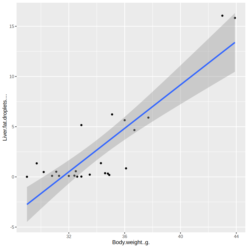
Not that good, as most of the mice have a small variation of liver fat droplets. As spearman’s correlation actually calculate the correlation based on the rank, let’s try another way to visualize:
library(ggplot2)
# draw
ggplot(data_for_plot, aes(x = rank(Body.weight..g.), y = rank(Liver.fat.droplets.... )) ) + # set the base
  geom_point(size = 1) +  # add  point
  stat_smooth(method = "lm",
              formula = y ~ x,
              geom = "smooth")
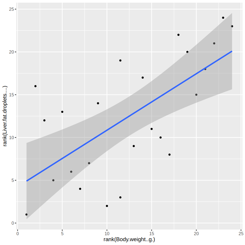
Great! You can see that the body weight and liver fat droplets do move in the same direction. And it is quite strong.
Case Exercise 9. Microbiota-wise correlation#
Previously, we have introduced how to do the correlation analysis on the metadata provided. Now, you are required to:
merge the otu_table with the meta_endpoint_data to form a dataframe that is ready to do correlation (hint: ?merge()).
Do correlation iteratively for each bacteria and each metadata (hint: Two for loop)
Store your results (most importantly your correlation coefficient and p value) in an R object for each association analysis, either a list() or a dataframe() (hint: create a new dataframe or list, and store your results within each of the for loop)
More Reading#
You may try other wrapper R packages, like microbiomeAnalyst.
Memorize the Great Contribution Made By the Giant#
Discovery of DNA#
1869: Friedrich Miescher discovered a substance he called “nuclein” (now known as DNA) in the nuclei of white blood cells.
1910s: Phoebus Levene identified the components of DNA as a phosphate-sugar-base structure, proposing the “tetranucleotide hypothesis.”
1944: Oswald Avery, Colin MacLeod, and Maclyn McCarty demonstrated that DNA is the molecule responsible for heredity in their transformation experiments with bacteria.
1950: Erwin Chargaff discovered that DNA composition varies between species and established Chargaff’s rules, noting that adenine equals thymine and guanine equals cytosine.
1952: Alfred Hershey and Martha Chase confirmed that DNA, not protein, is the genetic material using bacteriophage experiments.
1953: James Watson and Francis Crick, with critical contributions from Rosalind Franklin and Maurice Wilkins, proposed the double helix structure of DNA, revolutionizing biology.
Sequencing#
1977: Frederick Sanger developed the chain-termination method, known as Sanger sequencing, allowing for the rapid sequencing of DNA.
1980s-1990s: Automated sequencing machines were developed, increasing the speed and efficiency of DNA sequencing.
2001: The first draft of the Human Genome Project was completed using Sanger sequencing.
2005: Next-generation sequencing (NGS) technologies emerged, dramatically reducing the cost and time required for sequencing.
PCR (Polymerase Chain Reaction)#
1983: Kary Mullis invented PCR, a revolutionary technique allowing for the amplification of specific DNA sequences.
1985: The technique was first published, rapidly gaining popularity for its simplicity and effectiveness.
1990s: PCR became a fundamental tool in molecular biology, used in various applications such as cloning, diagnostics, and forensic science.
Cloning Techniques#
1972: Paul Berg performed the first successful gene splicing, laying the groundwork for cloning techniques.
1973: Herbert Boyer and Stanley Cohen developed a method for cloning DNA in bacteria using recombinant DNA technology.
1996: The first mammal, Dolly the sheep, was cloned from an adult somatic cell using somatic cell nuclear transfer (SCNT).
Common Technique Used in Molecular Biology#
Agarose Gel Electrophoresis: Arne Tiselius, a Swedish scientist who published his first study on electrophoresis. This technique separates DNA fragments based on size. By applying an electric current to a gel matrix, researchers could visualize and analyze DNA samples, allowing for the assessment of fragment length and purity.
Western blotting: A western blot experiment, or western blotting (also called immunoblotting, because an antibody is used to specifically detect its antigen) was introduced by Towbin, et al. in 1979 and is now a routine technique for protein analysis.
Restriction Enzyme Analysis: Restriction enzymes cut DNA at specific sequences, enabling scientists to analyze DNA fragments generated by these cuts. This method was crucial for mapping genomes and studying genetic variation.
Southern Blotting: Developed by Edwin Southern in 1975, this technique combines gel electrophoresis and hybridization. It allows for the detection of specific DNA sequences within a complex mixture, using labeled probes to identify complementary sequences.
Polymerase Chain Reaction (PCR): Invented in the 1980s, PCR enables the amplification of specific DNA segments, making it possible to study small amounts of DNA in detail. This technique revolutionized molecular biology and diagnostic testing.
DNA Probes and Hybridization: Researchers used labeled DNA probes to bind to complementary sequences in DNA samples, allowing for the identification of specific genes or mutations.
DNA Microarrays: Although more advanced than earlier methods, microarrays allowed for the simultaneous analysis of thousands of genes, providing insights into gene expression and regulation before the full sequencing of genomes.